AACE Methodology

The four classes of the CAPEX estimate

An estimate is not worth what it costs to prepare. It is worth what was known about the project when it was prepared. A reference guide to the AACE 18R-97 classification and how Kpex puts it to work.

Ca
Carlos Fuenmayor
Cost Engineer
· 21 Aug 2026 · 5 min read · 63 views
Back to Insights


CAF Engineering · Kpex Insight · Cost Engineering

The four classes of the CAPEX estimate

An estimate is not worth what it costs to prepare. It is worth what was known about the project when it was prepared. A reference guide to the AACE 18R-97 classification and how Kpex puts it to work.

The principle behind everything else

A persistent misconception runs through the industry: that an estimate is better because more hours went into it, better software produced it, or a more senior professional signed it. It is not. The quality of a capital cost estimate is governed, before anything else, by how mature the technical definition of the project was at the moment it was estimated.

That is the axis on which AACE International built Recommended Practice 18R-97, today the reference standard across the process industries. The classification does not describe how much effort was invested; it describes what was known. Three consequences follow in sequence: which methodology it is legitimate to apply, what accuracy range can honestly be promised, and which decision the resulting number is fit to support.

“Expected accuracy is not settled by consensus, nor inherited from a table. It is determined through risk analysis of the specific project — never by default.”

AACE International · RP 18R-97

Published ranges are calibration references, not promises. A poorly supported Class 3 estimate can behave like a Class 5. The reverse holds too: a robust cost database, with traceable sources and validated location factors, can carry a Class 4 to the favourable end of its band. The class sets the ceiling on what can be promised; the quality of the data decides where inside that ceiling you land.

Five classes, four investment decisions

The standard defines five classes, numbered counterintuitively: Class 5 is the earliest and least precise; Class 1 the most mature. The descending count follows the project life cycle — you start at 5 and work down towards 1 as engineering matures.

In owner practice, four of those five classes support real investment decisions: Class 5 to screen opportunities, Class 4 to select the option, Class 3 to authorise the budget, and Class 2 to control execution. Class 1 is a check estimate, normally prepared by the contractor with detailed engineering nearly complete, to validate a bid or price change orders. That is why Kpex structures its estimating engine around those four classes: they are the ones an owner's cost team runs repeatedly

The four classes, one by one

Each class has a methodology that belongs to it. Applying a higher class's method to a lower class's data does not improve the estimate — it only dresses uncertainty up as precision. What follows is what each class actually contains, and how Kpex executes it.

5

Screening · Order of Magnitude

Opportunity screening

Answers a single question: is this project worth spending engineering hours on? Produced when all that exists is a target capacity and a candidate technology.

−50% / +100%Accuracy range
0 – 2%Definition maturity
20 – 40%Typical contingency
Relative effort
Cost curves — capacity factored · Six-tenths rule
C = C_ref × (Q / Q_ref)n   where   n ≈ 0.6   (technology specific)

Capacity factoring exploits an empirical regularity of the process industries: the cost of a facility does not scale linearly with size, but with size raised to an exponent below one. Doubling capacity does not double cost; it multiplies it by roughly 1.5. That exponent n — the well-known six-tenths rule — is not universal. It varies by technology family, and getting its real value right is what separates a defensible screening estimate from a napkin.

In Kpex the process runs in three steps. You select the facility type and technology subfamily from the Module C taxonomy — each carries its own validated reference cost and exponent — enter a single sizing parameter (MW, bbl/day, t/yr, m²), then localise and escalate the result through the Z.4 (LFI) and Z.5 (CAI) indices. The output is a single TIC figure, not a breakdown.

Inputs required

  • Facility type
  • Technology subfamily
  • One capacity parameter (MW · bbl/day · t/yr)
  • Location and target date

Outputs produced

  • Order-of-magnitude TIC (single figure)
  • ±50–100% accuracy band
  • LFI + CAI adjusted total
Kpex modules appliedC — Facilities Cost ModelsZ.4 — CAF LFIZ.5 — CAF CAI
Characteristic risk: extrapolating the curve beyond its range of validity. A model calibrated between 50 and 500 MW says nothing reliable about 2 GW. Outside its range the exponent stops behaving, and the error runs well past the nominal +100%.
4

Study · Feasibility

Study and option selection

The class where configuration decisions are made. A process flow diagram and a preliminary equipment list now exist: the estimate stops being a figure and becomes a structure.

−30% / +50%Accuracy range
1 – 15%Definition maturity
15 – 25%Typical contingency
2–4×Relative effort
Equipment factored method — KPEX-HF · WBS breakdown
TIC = Σ ( C_eq × HF_family )

Here the facility stops being estimated as a whole and starts being estimated equipment by equipment. Each major item is priced from the Module A parametric curves (A.1.1 through A.1.5) by entering its sizing parameter — flow, heat transfer area, power, volume — and the curve returns a unit cost with its own accuracy band.

The KPEX-HF allowances then act on that bare equipment cost: installation factors by equipment family — compressors, pumps, heat exchangers, vessels, material handling, miscellaneous — that convert FOB cost into installed cost and distribute it across disciplines (civil, piping, E&I, erection). This is what separates modern factoring from the old Lang factor: each family has its own installation behaviour, and forcing them all through a single global multiplier builds a structural bias into the discipline split.

Kpex adds a layer the classical method lacks. The allowances are calibrated at P10/P50/P90, so the total is a distribution rather than a point. And the ARA tool (Z.6.5) weights the cost-source mix across all items — firm quote, OEM data, RFQ, parametric curve — to compute the accuracy actually achieved and test it against the expected Class 4 band. An estimate built mostly on firm quotes can therefore tighten its band in a way that is justified and traceable.

Inputs required

  • WBS structure: areas and functional units
  • Equipment list by family (Module A)
  • KPEX-HF family assignment per item
  • Declared cost source per item

Outputs produced

  • TIC with discipline-level breakdown
  • Factored total with P10/P50/P90 band
  • ARA accuracy rating (Z.6.5)
  • Basis of Estimate report (PDF)
Kpex modules appliedA — Process EquipmentKPEX-HFZ.4 — LFIZ.5 — CAIZ.6.5 — ARA
Critical point: the quality of a Class 4 estimate depends almost entirely on the equipment list being complete. Flawless factoring over a list missing three secondary items carries a scope error no factor can correct. Close the list before you fine-tune the factors.
3

Budget · Authorization

Budget and investment authorisation

The estimate that goes to the board. From here the figure stops informing and starts committing: it becomes the baseline against which project performance will be measured.

−20% / +30%Accuracy range
10 – 40%Definition maturity
10 – 20%Typical contingency
3–10×Relative effort
Module factor method · installation factor per item
Installed cost = Σ ( C_eq,i × f_module,i ) + Σ ( Q_discipline × unit_price )

The step up from Class 4 is granularity. Factoring no longer happens by equipment family but item by item: each piece of equipment carries its own module factor, sensitive to material of construction, design pressure, skid complexity and location within the plant. And discipline bulks — metres of pipe, m³ of concrete, metres of cable tray — stop being derived by factor and start being estimated by quantity, even if still on preliminary bases.

The distinctive contribution of this class is that contingency stops being a customary percentage. Kpex runs the PDRI tool (Z.6.3) — Project Definition Rating Index, in its industrial, infrastructure, buildings and oil & gas EPC variants — which scores the real maturity of the definition through a structured checklist of scope elements. That score translates directly into the recommended contingency percentage. A poor PDRI is not offset by optimism: it is paid for in contingency, or corrected by closing definition before going to the board.

Inputs required

  • Complete WBS: areas and functional units
  • Detailed equipment list with specifications
  • Bulk quantities by discipline
  • PDRI assessment score (Z.6.3)

Outputs produced

  • Full discipline cost breakdown
  • PDRI-calibrated contingency
  • Board-ready Basis of Estimate
  • Baseline for project control
Kpex modules appliedWBS BuilderA — Process EquipmentZ.2 — Construction LaborZ.3 — Rental EquipmentZ.6.3 — PDRI
The classic trap: presenting as Class 3 an estimate that only has Class 4 maturity, because the approval calendar would not wait. It is the documented origin of most severe CAPEX overruns — not a calculation failure, but a misdeclared class.
2

Control · Detailed

Control and execution

The deterministic estimate. It stops being a statistical prediction and becomes the sum of real line items: measured quantities, market prices and crew hours.

−15% / +20%Accuracy range
30 – 75%Definition maturity
5 – 10%Typical contingency
5–20×Relative effort
Quantity-based method (MTO) · deterministic
Cost = Σ ( quantity × unit_price ) + Σ ( crew_hours × Z.2_rate ) × PEI

Factors disappear here. Every line item comes from a real material take-off, priced with Module A unit prices and construction equipment rental rates from Z.3. Labour is calculated by crew with Z.2 rates, split by discipline and broken down by crew composition.

Two specific adjustments separate a rigorous Class 2 from an optimistic spreadsheet. The PEI (Z.6.2) — Productivity Efficiency Index — corrects labour output for real site conditions: weather, altitude, remoteness, congestion, availability of skilled trades, shift regime. Applying European reference productivities to a remote high-altitude site is one of the industry's most expensive and least visible mistakes. And the CRI (Z.6.4) — Construction Readiness Index — confirms the site is genuinely fit to mobilise: permits, access, released engineering, committed procurement.

The WBS stops being a grouping scheme and becomes control infrastructure: every measured quantity hangs from a specific cost account, which is what makes the S-curve, the milestone cash flow and later earned-value comparison possible.

Inputs required

  • WBS at full MTO depth
  • Equipment list with specs and vendor data
  • MTO quantities by discipline (m of pipe, m² formwork…)
  • Z.2 crew rates and PEI productivity index (Z.6.2)

Outputs produced

  • Full line-item cost breakdown
  • Milestone cash flow, S-curve ready
  • CRI-validated construction readiness (Z.6.4)
  • Contingency tied to the residual risk register
Kpex modules appliedWBS BuilderA — Process EquipmentZ.2 — Labor RatesZ.3 — Rental EquipmentZ.6.2 — PEIZ.6.4 — CRI
Where accuracy is lost: a Class 2 estimate rarely misses on materials. It misses on labour productivity and construction indirect hours. That is the chapter with the highest variance and, usually, the least attention.

Comparison matrix

All five classes in one view. Accuracy ranges correspond to the upper end of the bands published by AACE 18R-97 for the process industries; relative effort is an indicative index against a Class 5 estimate.

ClassDefinitionEnd usageMethodologyAccuracyConting.Effort
5Screening0 – 2%Portfolio screeningCapacity curves, parametric, analogy−50% / +100%20 – 40%
4Study1 – 15%Feasibility, option selectionEquipment factored (KPEX-HF)−30% / +50%15 – 25%2 – 4×
3Budget10 – 40%Investment authorisation, baselinePer-item module factors + bulks−20% / +30%10 – 20%3 – 10×
2Control30 – 75%Execution control, bid/tenderMTO quantities × unit prices−15% / +20%5 – 10%5 – 20×
1Check65 – 100%Bid validation, change ordersDetailed MTO, detailed engineering−10% / +15%3 – 5%10 – 100×

Class 1 is included for completeness of the standard; it falls outside the operating scope of Kpex, which is built around the owner's decision cycle.

Accuracy and contingency are not the same thing

This is the most widespread conceptual confusion in the field, and the one that generates the most unproductive argument in investment committees. It is worth separating precisely.

Contingency is money. It is a budgeted line, included in the estimate, covering what we know will happen but cannot yet identify item by item: scope growth within the current definition, normal execution inefficiency, quantity variability. An estimate with properly calculated contingency should be about as likely to fall short as to come in under — by construction, it is a P50.

The accuracy range is a probability. It describes how far the final cost may deviate from an estimate that already includes contingency. The standard is explicit on this point: the published ranges assume appropriate contingency has been applied. Without it, the real range is appreciably wider than the table's.

Contingency answers “how much money am I asking for?” Accuracy answers “how much confidence do I have in that figure?” Neither substitutes for the other, and adding contingency never improves the class.

Hence the operational value of working with distributions rather than points. KPEX-HF allowances calibrated at P10/P50/P90 allow you to state explicitly what confidence level the figure taken to the board represents, and the assessment tools — PDRI for Class 3 contingency, ARA for Class 4 accuracy, PEI and CRI for Class 2 execution risk — replace undocumented judgment with auditable criteria. Which is, in the end, the only thing that separates a professional estimate from a well-presented opinion.

Five expensive mistakes

  1. Declaring a class the definition does not supportThe dominant error. It is labelled Class 3 because the board meets on Thursday, not because there is 10% definition. The class is set by the state of engineering, never by the approval calendar. The PDRI exists precisely to make that check objective and hard to sidestep.
  2. Applying a method above the real classBuilding a detailed MTO on preliminary drawings does not produce a Class 2 estimate. It produces a Class 4 estimate that looks precise — far more dangerous, because nobody questions it. Method sophistication cannot exceed input data quality.
  3. Comparing estimates of different classesA Class 5 estimate of option A and a Class 3 estimate of option B are not comparable. The better-defined option almost always looks more expensive, simply because it has surfaced the costs the other is still hiding. Selection decisions require class parity.
  4. Ignoring location and escalationA reference cost without a location factor (LFI) or a time adjustment index (CAI) is data from another country and another year. On international projects the combined effect comfortably exceeds the full accuracy range of the class — more is lost here than in fine-tuning installation factors.
  5. Cutting contingency to make the number fitReducing contingency does not reduce cost. It only moves the overrun from the estimate to the closeout report. If the figure does not fit the available budget, the honest conversation is about scope, not about the percentage.

Which class do you need

Four questions settle almost every case. The right class is the cheapest one that supports the decision at hand — no less, and certainly no more.

Class 5

Is this worth a look?

Comparing portfolio opportunities, discarding quickly, setting an order of magnitude for a preliminary conversation. Days of work, not weeks.

Class 4

Which of these options?

Selecting technology, configuration or site. Needs comparability between alternatives and a discipline-level breakdown, not absolute accuracy.

Class 3

How much money do I ask for?

Investment authorisation and baseline setting. This is the figure that becomes a corporate commitment and the yardstick for the project.

Class 2

Are we on track?

Execution control, bid evaluation and change management. Requires line-item granularity and traceability down to the cost account.

Methodological note and sources

The accuracy ranges, definition maturity levels and methodologies cited here come from AACE International Recommended Practice 18R-97, Cost Estimate Classification System — As Applied in Engineering, Procurement, and Construction for the Process Industries. The ranges shown correspond to the upper end of the published bands. The relative effort index is indicative and takes a Class 5 estimate as its reference. Contingency percentages are typical industry guidance and must always be calibrated through risk analysis of the specific project.

The methodological implementation — Modules A, C and Z, KPEX-HF allowances and the LFI, CAI, PDRI, PEI, CRI and ARA assessment tools — corresponds to the Kpex platform by CAF Corporation Ingeniería de Costes.

  1. AACE International, RP 18R-97 — Cost Estimate Classification System for the Process Industries.
  2. AACE International, PGD-01 — Guide to Cost Estimate Classification Systems.
  3. Kpex — Official WBS structure v5, CAF Corporation Ingeniería de Costes SL.

CAF Engineering · Kpex — Project Cost Intelligence Platform · caf-corporation.com